WP4 – Task 4.3 Benchmarking tools to enhance computational performance of SAM
Romuald Hounyeme
14 avril 2026
Source:vignettes/Main_introductory_vignette_benchmarking.Rmd
Main_introductory_vignette_benchmarking.RmdGeneral introduction
Improving computational performance in Bayesian hierarchical models has become a central challenge in quantitative ecology and fisheries science, particularly for stock assessment workflows that require repeated, timely, and reproducible analyses. Although hierarchical Bayesian models provide major conceptual advantages—explicit separation of process and observation uncertainty, coherent propagation of uncertainty, flexible representation of latent ecological processes, and integration of heterogeneous multi-scale data—their practical deployment is frequently constrained by severe computational bottlenecks and fragile inference behavior (Brooks et al. 2011; Gelman et al. 2013). These limitations commonly manifest as long warm-up phases, unstable or divergent MCMC trajectories, poor exploration of high-dimensional posterior geometries, and diagnostics that become difficult to interpret at scale.
Hierarchical Bayesian approaches now underpin much of modern population dynamics inference, including Integrated Population Models (IPMs) (Besbeas et al. 2002; Royle and Kery 2016), Life Cycle Models (LCMs) (Caswell 2001; Ellner and Rees 2006), and State-Space Models (SSMs) (Kalman 1960; Stephen Terrence Buckland et al. 2004; Rivot et al. 2004). Their strength lies in combining information streams that are often incomplete, irregular, and collected at distinct spatial and temporal resolutions, while retaining a mechanistic interpretation of latent processes (Fieberg et al. 2010; Schaub and Abadi 2011). Such integrated approaches are fundamental for adaptive management, viability assessments, climate-impact attribution, and conservation planning (Nichols and Williams 2006; Jenouvrier et al. 2009; Zipkin and Saunders 2018).
However, Bayesian inference for these models still relies predominantly on MCMC algorithms whose efficiency can degrade rapidly under strong posterior correlations, non-linearities, weak identifiability, and high parameter dimensionality (Roberts and Rosenthal 1998; Carpenter et al. 2017). Motivated by these challenges, the work conducted within the European DIASPARA project (WP4, Task 4.3) developed a systematic framework to diagnose and improve computational performance for hierarchical Bayesian stock assessment models. This framework is implemented in the R package samOptiPro (v0.1.0) and is described in detail in an accompanying scientific manuscript.
The contribution of samOptiPro is to operationalize a unified workflow that combines:
-Automated structural diagnostics of model components (distributions, supports, truncations, differentiability constraints, dependency structure);
-Sampler selection without manual tuning, enabling principled use of HMC/NUTS, Slice-based methods, Random-Walk variants, and blocking strategies when appropriate;
-A bottleneck analysis pipeline to identify inefficient nodes and node families;
-Reproducible benchmarking of efficiency metrics, including Effective Sample Size (ESS) and derived measures of algorithmic and computational efficiency.
Scope of this vignette
This vignette is intentionally limited to a toy example, presented step by step to demonstrate the package workflow and the logic of the diagnostics and benchmarking outputs. The applied results for the operational case studies (i) the Scorff salmon LCM, (ii) the pan-Atlantic WGNAS LCM, and (iii) GEREM for European eel recruitment will be documented in separate vignettes, each dedicated to the corresponding model family and its optimization results.
DIASPARA project context and WP4
Amphihaline species such as European eel (Anguilla anguilla) and Atlantic salmon (Salmo salar) have complex life cycles spanning multiple environments and involving processes that are strongly modulated by environmental variability and human pressures. Sustainable management requires coherent integration of heterogeneous information streams—biological monitoring, fisheries data, counting facilities, and tagging programs—within modelling frameworks that quantify trends while rigorously propagating uncertainty (e.g., ICES advisory contexts) (Ahlbeck-Bergendahl et al. 2019; Rivot, Chaput, and Ensing 2021).
Within this landscape, DIASPARA aims to strengthen monitoring, understanding, and management of amphihaline populations through integrated modelling tools, robust indicators, and management scenario evaluation. Hierarchical Bayesian models are central to this effort because they naturally combine multiple data sources, represent latent biological processes explicitly, and provide principled uncertainty propagation—features widely recognized as critical in contemporary stock assessment practice (Maunder and Punt 2013; Punt et al. 2020).
Work Package 4 (WP4) focuses on enhancing stock assessment models from both ecological-structural and statistical-computational perspectives. The target models span SAMs, LCMs, and SSMs, and often involve deep spatio-temporal hierarchies, large latent state vectors, and complex dependencies between biological components (Stephen T. Buckland et al. 2004; Thorson et al. 2015). While such complexity increases biological realism and inferential coherence, it often yields posterior geometries that are high-dimensional, correlated, and sometimes weakly identified—conditions that can severely impair MCMC mixing and inflate computational cost (Brooks et al. 2011; Betancourt 2017).
Task 4.3 (“Benchmarking tools to enhance computational performance of SAM”) addresses these issues by providing a generic methodology to (i) detect computational bottlenecks, (ii) compare alternative sampling strategies (Random-Walk Metropolis, Slice sampling, HMC/NUTS, blocking, etc.), and (iii) quantify performance trade-offs in a reproducible way. A core premise is that one size does not fit all: optimal sampling strategies depend on model structure, posterior geometry, and differentiability constraints, and therefore must be selected and validated diagnostically rather than imposed universally. WP4 also aims to deliver practical, reusable tools and workflows to diagnose, configure, and benchmark MCMC algorithms in large integrated stock assessment models, thereby facilitating their adoption by assessment working groups.
Hierarchical Bayesian models and computational bottlenecks
Hierarchical Bayesian models are widely used in ecological and fisheries inference because they allow:
-integration of multiple heterogeneous data sources;
-explicit modelling of complex latent processes (e.g., recruitment, survival, migration, maturation);
-clear separation and propagation of uncertainty across process, observation, and parameter levels.
In practice, MCMC performance may deteriorate sharply when models become:
-strongly non-linear;
-high-dimensional;
-characterized by strong hierarchical dependencies and posterior correlations;
-built with distributions and constructs that are problematic for gradient-based methods (e.g., truncations, discrete components, hard constraints).
These difficulties typically lead to long runtimes, low ESS for key parameters, challenging convergence assessment (e.g., elevated ), and ultimately slower model-development and decision-support cycles.
Specific objectives of Task 4.3
Task 4.3 pursues four operational objectives:
-Diagnose structural and computational limitations of hierarchical Bayesian models used within DIASPARA and ICES-related workflows (including WGNAS).
-Develop generic tools to automatically detect computational bottlenecks at the level of nodes, node families, and dependency structures.
-Provide an automated pipeline to configure and benchmark MCMC sampling strategies (HMC, NUTS, Slice, Random-Walk variants, blocking), implemented in NIMBLE with nimbleHMC.
-Consolidate methods into an open-source R package (samOptiPro, v0.1.0) and a companion scientific manuscript describing design choices, methodology, and key results.
Scope of the present vignette
This vignette provides a practical, implementation-oriented introduction to the samOptiPro workflow using a toy model. The theoretical and methodological foundations are documented in the companion manuscript; the applied results for the Scorff LCM, WGNAS, and GEREM are presented in separate, model-specific vignettes.
Materials and Methods
Software ecosystem: NIMBLE, nimbleHMC, and samOptiPro
NIMBLE and nimbleHMC
All models considered in this work are implemented in NIMBLE, an R framework for specifying, compiling, and performing inference for hierarchical Bayesian models. NIMBLE combines BUGS-like model syntax with compilation of both models and inference algorithms, enabling fine-grained control over MCMC configuration and custom sampling strategies.
A key advantage of NIMBLE in the present context is its explicit access to model structure (nodes, dependency graphs, node families), which is essential for diagnosing differentiability constraints and designing targeted sampling interventions. The nimbleHMC package integrates Hamiltonian Monte Carlo (HMC) and the No-U-Turn Sampler (NUTS) into NIMBLE, enabling gradient-based sampling for compatible continuous components. These methods often improve algorithmic efficiency under strong posterior correlations, but require differentiable log densities—an assumption frequently violated in ecological models due to truncations, discrete distributions, and hard constraints (Betancourt 2017; Carpenter et al. 2017).
The samOptiPro package (v0.1.0)
Within Task 4.3, I developed samOptiPro to provide a coherent toolkit for diagnosing, optimizing, and benchmarking MCMC performance in complex NIMBLE models.
The package includes:
-structural diagnostic functions to assess compatibility with HMC/NUTS (automatic detection of non-differentiable constructs such as truncations, discrete components, conditional rules, and simplex-type constraints);
-scalable MCMC diagnostics for large parameter spaces (vectorized ESS and , and derived metrics of algorithmic and computational efficiency with aggregation by node families or biological components);
-automated sampler-configuration utilities, including:
-global HMC/NUTS attempts when structurally feasible;
-“surgical” strategies that target specific node families identified as bottlenecks (e.g., scalar or block NUTS/HMC, adaptive Slice variants, block Random-Walk), while keeping robust default samplers for the remainder.
General methodological pipeline
The analysis pipeline used for a given model is organized into five steps:
Step 1 — Model construction in NIMBLE. Each model is wrapped in a build_M()-type function returning at minimum: (i) a model object, (ii) an MCMC configuration conf, and (iii) optionally a set of monitors.
Step 2 — Preliminary structural diagnostics. An automated structural check is run (e.g., run_structure_and_hmc_test(build_fn, …)) to:
-count stochastic and deterministic nodes;
-detect potentially non-differentiable distributions/functions;
-identify explicit/implicit truncations and constraints;
-return a structural verdict regarding the feasibility of HMC/NUTS (globally or on subsets).
Step 3 — Baseline run. A default MCMC configuration (often RW + Slice) is used to:
-obtain initial MCMC chains;
-compute diagnostics and derived metrics (ESS, , AE, CE) using robust vectorized tooling (e.g., compute_diag_from_mcmc_vect_alt());
-identify low-CE node families as computational bottlenecks.
Step 4 — Sampler optimization strategies. Candidate strategies are tested (e.g., test_strategy(), test_strategy_family()):
-attempt global HMC/NUTS when feasible;
-otherwise, deploy targeted strategies on priority node families (e.g., scalar or block NUTS, AF_slice, RW_block), keeping robust defaults elsewhere.
Step 5 — Performance comparison and interpretation. Optimized configurations are compared to the baseline:
-parameter- and family-level comparisons (ESS, , AE, CE);
-diagnostic visualizations (CE profiles, ESS distributions, convergence diagnostics);
-interpretation of gains in relation to model structure and dependency geometry.
A representative pseudo-code for this pipeline, together with a step-by-step demonstration, is provided below using a toy example. # Tutorial
This tutorial demonstrates how to diagnose
differentiability and optimize MCMC sampling
strategies in complex Bayesian state–space models using the R
package samOptiPro (Hounyeme et
al., 2025).
We illustrate the workflow on a simple population dynamics model, using
nimble and nimbleHMC as the computational
back-end.
We will:
- Build and simulate a population growth model with a
latent process and log-normal observations.
- Identify bottlenecks (algorithmic bottlenecks and time
bottlenecks).
- Diagnose non-differentiable components (to decide
whether HMC/NUTS is applicable).
- Automatically benchmark samplers (RW, slice,
AF_slice, HMC, NUTS) using
test_strategy_family()/test_strategy().
- Assess algorithmic efficiency (AE) and computational efficiency (CE).
All results (traceplots, diagnostics, and performance summaries) are
saved under outputs/.
Step 0 – Load packages
nimble version 1.4.2 is loaded.
For more information on NIMBLE and a User Manual,
please visit https://R-nimble.org.
Attaching package: 'nimble'The following object is masked from 'package:stats':
simulateThe following object is masked from 'package:base':
declare
library(nimbleHMC)Step 1 – Simulated data, initial values and monitors
# Simulation constants
time <- 8
Const_nimble <- list(
  n        = time,
  sd_obs   = c(0.05, rep(0.4, time - 1))
)

# Data simulation
set.seed(42)
Nobs  <- numeric(time)
theta <- numeric(time - 1)
Nobs[1] <- rlnorm(1, meanlog = 10, sdlog = 0.5)

for (t in 1:(time - 1)) {
  theta[t]  <- runif(1, 0.7, 0.9)
  Nobs[t+1] <- Nobs[t] * theta[t]
}

Data_nimble <- list(Nobs = Nobs)

# Initial values
Inits_nimble <- list(
  N           = 2e4 * c(1, cumprod(rep(0.8, time - 1))),
  logit_theta = rep(logit(0.8), time - 1)
)

# Monitors
monitors <- c("N", "theta", "logit_theta")
Step 2 – Model M3
M3.nimble <- nimbleCode({
  # priors
  for (t in 1:(n-1)) {
    logit_theta[t] ~ dnorm(mean = 2, sd = 1)
    theta[t] <- ilogit(logit_theta[t])
  }
  N[1] ~ dlnorm(meanlog = 10, sdlog = 5)

  # process model
  for (t in 1:(n-1)) {
    N[t+1] <- N[t] * theta[t]
  }

  # observation model
  Nobs[1] ~ dlnorm(meanlog = log(N[1]), sdlog = sd_obs[1])
  for (t in 3:n) {
    Nobs[t] ~ dlnorm(meanlog = log(N[t]), sdlog = sd_obs[t])
  }
})
Step 3 – Building and compiling the model
The function build_M() is the central entry point used
by most samOptiPro tools. It returns the model, its
compiled version, the default monitors and the model code as plain
text.
nimbleOptions(buildInterfacesForCompiledNestedNimbleFunctions = TRUE)
nimbleOptions(MCMCsaveHistory = FALSE)

m <- nimbleModel(
  code        = M3.nimble,
  name        = "M3",
  constants   = Const_nimble,
  data        = Data_nimble,
  inits       = Inits_nimble,
  buildDerivs = TRUE
)
Defining modelBuilding modelSetting data and initial valuesRunning calculate on model
[Note] Any error reports that follow may simply reflect missing values in model variables.Checking model sizes and dimensions [Note] This model is not fully initialized. This is not an error.
To see which variables are not initialized, use model$initializeInfo().
For more information on model initialization, see help(modelInitialization).
cm <- compileNimble(m)Compiling
[Note] This may take a minute.
[Note] Use 'showCompilerOutput = TRUE' to see C++ compilation details.Step 4 – Diagnosing differentiability and HMC eligibility
diagnose_model_structure(): structural and timing
bottlenecks
The function diagnose_model_structure() inspects the
graph structure of a NIMBLE model and returns a set of
tables describing:
- the list of stochastic and deterministic nodes;
- the dependency graph (downstream nodes for each variable);
- a decomposition of node families (e.g.
logit_theta,N,theta) and their dependency counts;
- optional timing information for samplers (via an internal profiling run).
Conceptually, diagnose_model_structure() is
purely structural: it only needs a compiled model, not
MCMC samples. It is therefore cheap and can be used early, even before
running any long MCMC.
In practice, we call it as follows for the M3 model:
cat("\n[MODEL STRUCTURE CHECK]\n")
[MODEL STRUCTURE CHECK]
#by family
diag_s <- diagnose_model_structure(
  model              = m,
  include_data       = FALSE,
  removed_nodes      = NULL,
  ignore_patterns    = c("^lifted_", "^logProb_"),
  make_plots         = TRUE,
  output_dir         = "outputs/diagnostics",
  save_csv           = FALSE,
  node_of_interest   = NULL,
  sampler_times      = NULL,
  sampler_times_unit = "seconds",
  auto_profile       = TRUE,
  profile_niter      = 2200,
  profile_burnin     = 500,
  profile_thin       = 1,
  profile_seed       = NULL,
  np                 = 1,
  by_family          = TRUE,
  family_stat        = c("median", "mean", "sum"),
  time_normalize     = c("none", "per_node"),
  only_family_plots  = TRUE
)
[TIME] Get all node names ...
[TIME] Get all node names: user=0.000s, sys=0.000s, elapsed=0.001s

[TIME] Filter ignore patterns and removed_nodes ...
[TIME] Filter ignore patterns and removed_nodes: user=0.000s, sys=0.000s, elapsed=0.000s

[TIME] Get stochastic node names ...
[TIME] Get stochastic node names: user=0.000s, sys=0.000s, elapsed=0.001s

[STRUCTURE]
- # stochastic nodes   : 8
- # deterministic nodes: 14

[TIME] getVarInfo() over base variables ...
[TIME] getVarInfo() over base variables: user=0.000s, sys=0.000s, elapsed=0.001s

[TIME] Compute dependencies for all base nodes (memoized) ...
[TIME] Compute dependencies for all base nodes (memoized): user=0.026s, sys=0.000s, elapsed=0.026s

[TIME] nimble::configureMCMC(model, ...) ...
===== Monitors =====
thin = 1: logit_theta, N
===== Samplers =====
RW sampler (8)
  - logit_theta[]  (7 elements)
  - N[]  (1 element)
[TIME] nimble::configureMCMC(model, ...): user=0.124s, sys=0.001s, elapsed=0.125s

[TIME] Extract samplers and targets ...
[TIME] Extract samplers and targets: user=0.002s, sys=0.000s, elapsed=0.002s

[TIME] Auto-profile samplers (internal MCMC run) ...
Compiling
[Note] This may take a minute.
[Note] Use 'showCompilerOutput = TRUE' to see C++ compilation details.|-------------|-------------|-------------|-------------|
|-------------------------------------------------------|
[PROFILE] Raw sampler_times length (internal) = 8.
[TIME] Auto-profile samplers (internal MCMC run): user=2.165s, sys=0.033s, elapsed=7.112s
[TIME] Aggregate sampler times per parameter ...
[TIME] Aggregate sampler times per parameter: user=0.003s, sys=0.000s, elapsed=0.003s
[TIME] Assemble deps_df (node order by total_dependencies) ...
[TIME] Assemble deps_df (node order by total_dependencies): user=0.001s, sys=0.000s, elapsed=0.000s
[TIME] Assemble sampler_df (restricted to nodes with sampler) ...
[TIME] Assemble sampler_df (restricted to nodes with sampler): user=0.001s, sys=0.000s, elapsed=0.000s
[TIME] Compute node_of_interest downstream ...
[TIME] Compute node_of_interest downstream: user=0.000s, sys=0.000s, elapsed=0.000s
[TIME] Aggregate dependencies by family ...
[TIME] Aggregate dependencies by family: user=0.001s, sys=0.000s, elapsed=0.001s
[TIME] Aggregate sampler time by family ...
[TIME] Aggregate sampler time by family: user=0.001s, sys=0.000s, elapsed=0.001s
[TIME] Make plots ...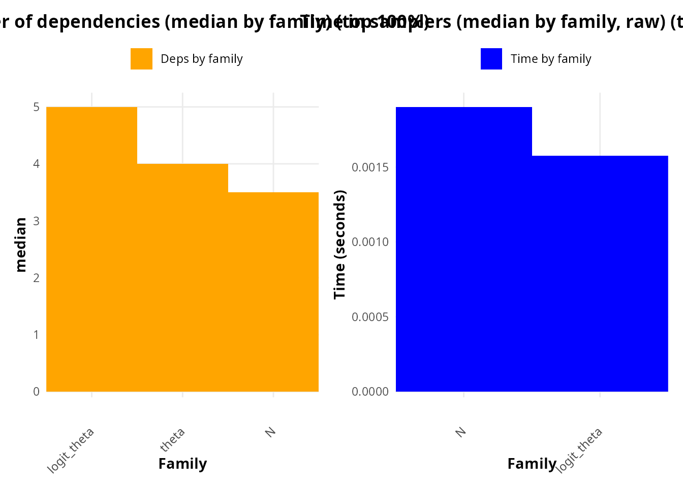
[TIME] Make plots: user=1.464s, sys=0.034s, elapsed=1.500s

[TIME] Assemble return object ...
[TIME] Assemble return object: user=0.000s, sys=0.000s, elapsed=0.000s
#by node
diag_s <- diagnose_model_structure(
  model              = m,
  include_data       = FALSE,
  removed_nodes      = NULL,
  ignore_patterns    = c("^lifted_", "^logProb_"),
  make_plots         = TRUE,
  output_dir         = "outputs/diagnostics",
  save_csv           = FALSE,
  node_of_interest   = NULL,
  sampler_times      = NULL,
  sampler_times_unit = "seconds",
  auto_profile       = TRUE,
  profile_niter      = 2200,
  profile_burnin     = 500,
  profile_thin       = 1,
  profile_seed       = NULL,
  np                 = 1,
  by_family          = FALSE,
  family_stat        = c("median", "mean", "sum"),
  time_normalize     = c("none", "per_node"),
  only_family_plots  = TRUE
)
[TIME] Get all node names ...
[TIME] Get all node names: user=0.000s, sys=0.000s, elapsed=0.001s

[TIME] Filter ignore patterns and removed_nodes ...
[TIME] Filter ignore patterns and removed_nodes: user=0.000s, sys=0.000s, elapsed=0.000s

[TIME] Get stochastic node names ...
[TIME] Get stochastic node names: user=0.001s, sys=0.000s, elapsed=0.000s

[STRUCTURE]
- # stochastic nodes   : 8
- # deterministic nodes: 14

[TIME] getVarInfo() over base variables ...
[TIME] getVarInfo() over base variables: user=0.001s, sys=0.000s, elapsed=0.000s

[TIME] Compute dependencies for all base nodes (memoized) ...
[TIME] Compute dependencies for all base nodes (memoized): user=0.007s, sys=0.000s, elapsed=0.006s

[TIME] nimble::configureMCMC(model, ...) ...
===== Monitors =====
thin = 1: logit_theta, N
===== Samplers =====
RW sampler (8)
  - logit_theta[]  (7 elements)
  - N[]  (1 element)
[TIME] nimble::configureMCMC(model, ...): user=0.115s, sys=0.000s, elapsed=0.115s

[TIME] Extract samplers and targets ...
[TIME] Extract samplers and targets: user=0.002s, sys=0.000s, elapsed=0.002s

[TIME] Auto-profile samplers (internal MCMC run) ...
Compiling
[Note] This may take a minute.
[Note] Use 'showCompilerOutput = TRUE' to see C++ compilation details.[PROFILE] Raw sampler_times length (internal) = 8.
[TIME] Auto-profile samplers (internal MCMC run): user=2.282s, sys=0.010s, elapsed=7.234s
[TIME] Aggregate sampler times per parameter ...
[TIME] Aggregate sampler times per parameter: user=0.001s, sys=0.000s, elapsed=0.002s
[TIME] Assemble deps_df (node order by total_dependencies) ...
[TIME] Assemble deps_df (node order by total_dependencies): user=0.001s, sys=0.000s, elapsed=0.000s
[TIME] Assemble sampler_df (restricted to nodes with sampler) ...
[TIME] Assemble sampler_df (restricted to nodes with sampler): user=0.001s, sys=0.000s, elapsed=0.000s
[TIME] Compute node_of_interest downstream ...
[TIME] Compute node_of_interest downstream: user=0.000s, sys=0.000s, elapsed=0.000s
[TIME] Aggregate dependencies by family ...
[TIME] Aggregate dependencies by family: user=0.001s, sys=0.000s, elapsed=0.001s
[TIME] Aggregate sampler time by family ...
[TIME] Aggregate sampler time by family: user=0.001s, sys=0.000s, elapsed=0.002s
[TIME] Make plots ...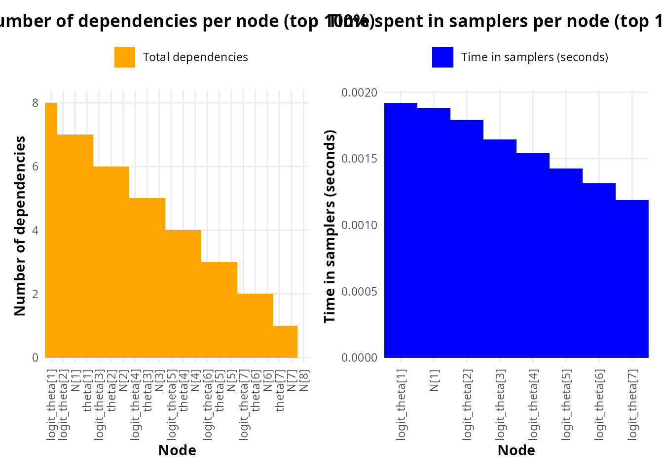
[TIME] Make plots: user=1.356s, sys=0.005s, elapsed=1.362s

[TIME] Assemble return object ...
[TIME] Assemble return object: user=0.000s, sys=0.000s, elapsed=0.000s
Structural dependencies and sampler time: identification of candidate bottlenecks
The structural diagnostic highlights a clear contrast between dependency structure and effective computational cost at different aggregation levels (family vs. node).
At the family level, the logit_theta family exhibits the highest median number of downstream dependencies, exceeding those of theta and N (Fig. X, top-left). This indicates that changes in logit_theta propagate broadly through the model graph, affecting a large number of deterministic and stochastic nodes. From a structural perspective, this family therefore represents a strong candidate for computational bottlenecks.
However, when considering median sampler time aggregated by family (Fig. X, top-right), logit_theta does not dominate as clearly as expected. Instead, the family-level aggregation smooths out heterogeneity among individual parameters, partially masking localized computational hotspots.
This discrepancy becomes explicit at the node level. The per-node dependency analysis (Fig. X, bottom-left) confirms that individual logit_theta[i] nodes—particularly logit_theta[1] and logit_theta[2]—are among the most connected nodes in the model. Crucially, the time spent in samplers per node (Fig. X, bottom-right) shows that these same nodes also incur the highest individual sampler costs, consistent with their structural position.
Taken together, these results support two important conclusions:
Family-level summaries alone are insufficient to identify computational bottlenecks, as they can obscure strong heterogeneity within parameter families.
Node-level diagnostics reveal localized bottlenecks, here concentrated in the first logit_theta components, which combine high dependency counts with elevated sampler time.
These observations motivate a first working hypothesis:
The earliest logit_theta nodes constitute primary computational bottlenecks and represent priority targets for sampler optimization (e.g. alternative samplers, blocking, or gradient-based methods), even when family-level summaries appear moderate.
This example illustrates the practical value of combining structural dependency diagnostics with fine-grained sampler-time profiling. In particular, it demonstrates why bottleneck identification in hierarchical Bayesian models should operate at multiple scales (family and node), rather than relying on aggregated metrics alone.
run_structure_and_hmc_test(): combined structure +
HMC/NUTS check
In practice, run_structure_and_hmc_test() is a
convenience wrapper: it calls diagnose_model_structure()
and, when possible, attempts a full‑model HMC/NUTS
configuration. This gives, in a single object out,
both the structural bottlenecks and an early indication of whether a
global HMC strategy is realistic for the current model.
out <- run_structure_and_hmc_test(build_M, include_data = FALSE)
[STRUCTURE]
- # stochastic nodes   : 8
- # deterministic nodes: 21

[NON-DIFF INDICATORS]
- Non-diff functions detected (present_in_code): None
- Non-diff functions detected (active_graph_given_constants): None
- Fatal (strict) non-diff functions detected: None
- Distributions found in code : dlnorm, dnorm
- BUGS-style truncation 'T(a,b)' spotted: No
- Bounded latent nodes (implicit truncation via finite bounds on continuous support): No

[HMC/NUTS SHOWSTOPPERS]
- No explicit showstoppers detected at latent nodes.

- Structurally suitable for HMC/NUTS? Yes

[HMC/NUTS SMOKE TEST]
===== Monitors =====
thin = 1: logit_theta, N
===== Samplers =====
RW sampler (8)
  - logit_theta[]  (7 elements)
  - N[]  (1 element)
thin = 1: logit_theta, N, theta
- HMC/NUTS empirical test: PASSEDStructural differentiability check and HMC/NUTS feasibility
We first apply run_structure_and_hmc_test(build_M, include_data = FALSE) to assess whether the toy model satisfies the differentiability requirements needed for gradient-based samplers (HMC/NUTS). The structural report indicates a compact graph (8 stochastic nodes; 21 deterministic nodes) and, critically, no detected non-differentiable constructs: no round/floor/piecewise indicators, no discrete distributions, and no BUGS-style truncation (T(a,b)). The only distributions detected in the model code are continuous and differentiable (dlnorm, dnorm), and no bounded latent nodes were flagged as implicitly truncated by finite support constraints.
Accordingly, no latent-node “showstoppers” were detected, and the model is classified as structurally suitable for HMC/NUTS. This conclusion is further supported by an empirical smoke test, which successfully runs a short HMC/NUTS configuration on the monitored latent components (logit_theta, N, and theta). Taken together, the structural scan and the smoke test provide practical evidence that the model’s log-posterior is compatible with gradient-based sampling, thereby justifying subsequent benchmarking of HMC/NUTS against slice- and random-walk–based alternatives. # Step 5 – Baseline MCMC, bottlenecks and performance assessment
run_baseline_config(): a safe default MCMC runner
run_baseline_config() is the main entry point to run a
baseline NIMBLE configuration on a given model:
- it calls your model builder (here
build_M());
- it configures a default sampler strategy (typically scalar RW,
possibly with default slice samplers);
- it compiles the MCMC and runs it for the requested number of
iterations and chains;
- it returns the raw samples together with the total runtime.
In this vignette, we use it to generate a long baseline run for model
M3. Because this can be time‑consuming, we mark the chunk as
eval = FALSE so that the vignette compiles quickly while
still showing the full code.
## MCMC schedule for the baseline run
n.iter   <- 1e6
n.burnin <- 1e4
n.thin   <- 2
n.chains <- 3

## Baseline configuration and run
res_a <- run_baseline_config(
  build_fn = build_M,
  niter    = n.iter,
  nburnin  = n.burnin,
  thin     = n.thin,
  nchains  = n.chains,
  monitors = monitors
)
===== Monitors =====
thin = 2: logit_theta, N, theta
thin2 = 1: logit_theta, N
===== Samplers =====
RW sampler (8)
- logit_theta[] (7 elements)
- N[] (1 element)
thin = 2: logit_theta, N, theta
thin2 = 1: logit_theta, N
thin = 2: logit_theta, N, theta
thin2 = 2: logit_theta, NCompiling
[Note] This may take a minute.
[Note] Use 'showCompilerOutput = TRUE' to see C++ compilation details.running chain 1...running chain 2...running chain 3...
## Merge samples / samples2 into a clean mcmc.list
samples_mla <- as_mcmc_list_sop(
  res_a$samples,
  res_a$samples2,
  drop_loglik = FALSE,
  thin        = n.thin
)

runtime_s_a <- res_a$runtime_s

## High-level performance summary
ap <- assess_performance(samples = samples_mla, runtime_s = runtime_s_a)

## Node-level bottlenecks
bot <- identify_bottlenecks(
  samples             = samples_mla,
  runtime_s           = runtime_s_a,
  ess_threshold       = 1000,
  sampler_params      = NULL,
  model               = m,
  mcmc_conf           = NULL,
  ignore_patterns     = c("^lifted_", "^logProb_"),
  strict_sampler_only = TRUE,
  auto_configure      = TRUE,
  rhat_threshold      = 1.01,
  ess_per_s_min       = 0
)
===== Monitors =====
thin = 1: logit_theta, N
===== Samplers =====
RW sampler (8)
- logit_theta[] (7 elements)
- N[] (1 element)
## Family-level bottlenecks
bot2 <- identify_bottlenecks_family(
  samples             = samples_mla,
  runtime_s           = runtime_s_a,
  ess_threshold       = 1000,
  sampler_params      = NULL,
  model               = m,
  mcmc_conf           = NULL,
  ignore_patterns     = c("^lifted_", "^logProb_"),
  strict_sampler_only = TRUE,
  auto_configure      = TRUE,
  rhat_threshold      = 1.01,
  ess_per_s_min       = 0
)
===== Monitors =====
thin = 1: logit_theta, N
===== Samplers =====
RW sampler (8)
- logit_theta[] (7 elements)
- N[] (1 element)
## --- Explicit printing (ensures Word/HTML output) ---
cat("\n--- Baseline runtime (s) ---\n")
--- Baseline runtime (s) ---
print(runtime_s_a)[1] 12.962
cat("\n--- Global performance summary ---\n")
--- Global performance summary ---
print(ap$summary)
[38;5;246m# A tibble: 1 × 12
[39m
  runtime_s n_chains n_iter n_draws_total n_params ESS_total ESS_per_s AE_mean AE_median

[3m
[38;5;246m<dbl>
[39m
[23m
[3m
[38;5;246m<int>
[39m
[23m
[3m
[38;5;246m<int>
[39m
[23m
[3m
[38;5;246m<int>
[39m
[23m
[3m
[38;5;246m<int>
[39m
[23m
[3m
[38;5;246m<dbl>
[39m
[23m
[3m
[38;5;246m<dbl>
[39m
[23m
[3m
[38;5;246m<dbl>
[39m
[23m
[3m
[38;5;246m<dbl>
[39m
[23m

[38;5;250m1
[39m      13.0        3
[4m4
[24m
[4m9
[24m
[4m5
[24m000       1
[4m4
[24m
[4m8
[24m
[4m5
[24m000       37 20
[4m6
[24m
[4m6
[24m
[4m9
[24m781.  1
[4m5
[24m
[4m9
[24m
[4m4
[24m644.   0.376     0.324

[38;5;246m# ℹ 3 more variables: CE_mean <dbl>, CE_median <dbl>, prop_rhat_ok <dbl>
[39m
cat("\n--- Worst nodes (top 3) ---\n")
--- Worst nodes (top 3) ---
print(bot$top3) axis parameter ESS CE AE slow_node_time CE_rank AE_rank
1 AE logit_theta[2] 359219.3 27713.26 0.2418985 0.03608381 1 1
2 AE logit_theta[1] 360302.8 27796.85 0.2426281 0.03597530 3 3
3 CE logit_theta[2] 359219.3 27713.26 0.2418985 0.03608381 1 1
4 CE logit_theta[1] 360302.8 27796.85 0.2426281 0.03597530 3 3
5 time logit_theta[2] 359219.3 27713.26 0.2418985 0.03608381 1 1
6 time logit_theta[1] 360302.8 27796.85 0.2426281 0.03597530 3 3
TIME_rank
1 1
2 3
3 1
4 3
5 1
6 3
cat("\n--- Worst families (top 3) ---\n")
--- Worst families (top 3) ---
print(bot2$top3) axis family n_members CE_med AE_med slow_node_time CE_rank AE_rank TIME_rank
1 AE logit_theta 7 32421.50 0.2829949 0.03084373 1 1 1
2 AE N 1 44939.41 0.3922590 0.02225218 2 2 2
3 CE logit_theta 7 32421.50 0.2829949 0.03084373 1 1 1
4 CE N 1 44939.41 0.3922590 0.02225218 2 2 2
5 time logit_theta 7 32421.50 0.2829949 0.03084373 1 1 1
6 time N 1 44939.41 0.3922590 0.02225218 2 2 2The baseline RW run confirms that computational inefficiency concentrates in the logit_theta family, with logit_theta[1] and logit_theta[2] emerging as the primary bottleneck nodes, consistent with the dependency/time profiling shown earlier.
Summary. The object res_a returned by
run_baseline_config() is then the baseline
reference for the whole pipeline:
-
samples,samples2are the raw draws used to derive ESS and R-hat;
-
runtime_sis the total runtime used to compute computational efficiency;
- downstream tools such as
assess_performance(),identify_bottlenecks()andidentify_bottlenecks_family()reuse these outputs to locate structural and algorithmic bottlenecks in model M3.
Step 6 – Adaptive block strategy:
test_strategy_family() and
test_strategy()
test_strategy_family(): surgical strategy search by
family
The core function of the optimisation pipeline is
test_strategy_family(). Given a family of
parameters (e.g. logit_theta) and a baseline run,
it:
- inspects the current samplers used for this family;
- proposes alternative samplers (e.g. scalar slice or block-wise
NUTS);
- runs short pilot chains under each strategy;
- compares per-parameter ESS, AE and CE against the baseline;
- returns a structured object that can be further plotted or summarised.
In the M3 toy example, one can use the legacy interface as:
knitr::opts_chunk$set(
  message = FALSE,
  warning = FALSE,
  echo    = FALSE,      # vignette-friendly: show results, not all code
  results = "markup"
)

# Quiet evaluator: suppress stdout/messages/warnings, keep returned objects
quiet_run <- function(expr) {
  tmp <- tempfile(fileext = ".log")
  zz  <- file(tmp, open = "wt")

  on.exit({
    try(sink(NULL), silent = TRUE)
    try(sink(NULL, type = "message"), silent = TRUE)
    try(close(zz), silent = TRUE)
  }, add = TRUE)

  sink(zz)
  sink(zz, type = "message")

  withCallingHandlers(
    expr,
    warning = function(w) invokeRestart("muffleWarning"),
    message = function(m) invokeRestart("muffleMessage")
  )
}

# Helper: % change as requested: (baseline - strategy)/baseline * 100
pct_change <- function(baseline, strategy) {
  ifelse(is.finite(baseline) && baseline != 0,
         (baseline - strategy) / baseline * 100,
         NA_real_)
}

fmt_pct <- function(x, digits = 1) {
  ifelse(is.na(x), NA_character_, sprintf("%+.1f%%", round(x, digits)))
}
# -------------------------------------------------------------------
# 0) Baseline summary is assumed already available in your workflow.
#     If baseline is produced elsewhere in the vignette, just store it
#     as a small list/data.frame used below (baseline_global, baseline_family).
# -------------------------------------------------------------------
# Example placeholders (replace with your actual stored baseline objects):
# baseline_global <- list(runtime_s = 19.372, AE_median = 0.3245393, CE_median = 28928.1)
# baseline_family <- data.frame(family=c("logit_theta","N"), AE_med=c(0.2854590,0.3907365), CE_med=c(21882.44,29952.70))

# -------------------------------------------------------------------
# 1) Short benchmark: full-model HMC/NUTS (guarded)
# -------------------------------------------------------------------
diff <- quiet_run(
  configure_hmc_safely(
    build_fn  = build_M,
    niter     = n.iter,
    nburnin   = n.burnin,
    thin      = n.thin,
    monitors  = monitors,
    nchains   = n.chains,
    out_dir   = "outputs/diagnostics"
  )
)
[1m
[33mError
[39m in `parse(text = x, keep.source = FALSE)[[1]]`:
[22m

[33m!
[39m subscript out of bounds
# -------------------------------------------------------------------
# 2) Family-focused pilot: Slice on bottleneck family (keep vignette light)
#    Use small defaults; describe larger runs in text.
# -------------------------------------------------------------------
diff1 <- quiet_run(
  test_strategy_family(
    build_fn               = build_M,
    monitors               = NULL,
    try_hmc                = TRUE,
    nchains                = n.chains,
    pilot_niter            = 1e6,     # vignette-friendly
    pilot_burnin           = 1e4,     # vignette-friendly
    thin                   = n.thin,
    out_dir                = "outputs/diagnostics",
    nbot                   = 1,
    strict_scalar_seq      = c("slice"),
    strict_block_seq       = c("NUTS_block", "AF_slice", "RW_block"),
    ask                    = FALSE,
    ask_before_hmc         = FALSE,
    block_max              = 20,
    slice_control          = list(),
    rw_control             = list(),
    rwblock_control        = list(adaptScaleOnly = TRUE),
    af_slice_control       = list(),
    slice_max_contractions = 5000
  )
)
# -----------------------------
# PUBLISHABLE OUTPUTS
# -----------------------------

# ---- 1) Global summary for full NUTS ----
cat("\n## Short benchmark: full-model HMC/NUTS (guarded)\n")
## Short benchmark: full-model HMC/NUTS (guarded)
runtime_nuts <- if (!is.null(diff$res$runtime_s)) diff$res$runtime_s else NA_real_
[1m
[33mError
[39m in `diff$res`:
[22m

[33m!
[39m object of type 'closure' is not subsettable
AE_med_nuts <- NA_real_
CE_med_nuts <- NA_real_
Rhat_max    <- NA_real_

if (!is.null(diff$diag_tbl) &&
    all(c("AE_ESS_per_it", "ESS_per_sec", "Rhat") %in% names(diff$diag_tbl))) {
  AE_med_nuts <- stats::median(diff$diag_tbl$AE_ESS_per_it, na.rm = TRUE)
  CE_med_nuts <- stats::median(diff$diag_tbl$ESS_per_sec,   na.rm = TRUE)
  Rhat_max    <- suppressWarnings(max(diff$diag_tbl$Rhat, na.rm = TRUE))
}
[1m
[33mError
[39m in `diff$diag_tbl`:
[22m

[33m!
[39m object of type 'closure' is not subsettable
**Runtime (s):**
[1m
[33mError
[39m:
[22m

[33m!
[39m object 'runtime_nuts' not found
cat("\n**Key summary:**\n")
**Key summary:**
print(data.frame(AE_median = AE_med_nuts, CE_median = CE_med_nuts, Rhat_max = Rhat_max)) AE_median CE_median Rhat_max
1 NA NA NA
# Optional: show only the bottleneck family head (avoid flooding vignette)
if (!is.null(diff$diag_tbl)) {
  cat("\n**Diagnostics (first 10 rows):**\n")
  print(utils::head(diff$diag_tbl, 10))
}
[1m
[33mError
[39m in `diff$diag_tbl`:
[22m

[33m!
[39m object of type 'closure' is not subsettable
# ---- 2) Extract Slice result restricted to logit_theta family ----
cat("\n## Family-focused pilot: Slice on bottleneck family\n")
## Family-focused pilot: Slice on bottleneck family
slice_tbl <- NULL
slice_runtime <- NA_real_

if (!is.null(diff1$steps) && length(diff1$steps) >= 1 &&
    !is.null(diff1$steps[[1]]$res)) {

  step1 <- diff1$steps[[1]]$res
  slice_runtime <- if (!is.null(step1$out$runtime_s)) step1$out$runtime_s else NA_real_

  if (!is.null(step1$dg)) {
    slice_tbl <- step1$dg
  }
}

if (!is.null(slice_tbl)) {
  # Keep only the bottleneck family
  slice_logit <- slice_tbl[slice_tbl$Family %in% "logit_theta", , drop = FALSE]
  cat("\n**Slice results on `logit_theta` (first rows):**\n")
  print(utils::head(slice_logit, 10))
} else {
  cat("\n(Info) Could not locate step diagnostics table in diff1.\n")
}
**Slice results on `logit_theta` (first rows):**
           target      ESS AE_ESS_per_it ESS_per_sec time_s_per_ESS     Rhat      Family
9  logit_theta[1] 406322.6     0.8208537    13537.77  0.00007386742 1.000003 logit_theta
10 logit_theta[2] 404696.5     0.8175687    13483.59  0.00007416422 1.000002 logit_theta
11 logit_theta[3] 428000.1     0.8646466    14260.01  0.00007012615 1.000004 logit_theta
12 logit_theta[4] 451607.8     0.9123389    15046.57  0.00006646033 1.000001 logit_theta
13 logit_theta[5] 479417.8     0.9685208    15973.14  0.00006260510 1.000001 logit_theta
14 logit_theta[6] 491981.0     0.9939010    16391.72  0.00006100642 1.000001 logit_theta
15 logit_theta[7] 492440.2     0.9948287    16407.02  0.00006094953 1.000000 logit_theta
# ---- 3) Summary tables with % change (baseline vs strategies) ----
# You must provide baseline_global & baseline_family from your baseline run.
# Here we only show the computation pattern.
if (exists("baseline_global", inherits = TRUE)) {

  tab_global <- data.frame(
    Metric = c("Runtime (s)", "AE_median", "CE_median (ESS/s)"),
    Baseline = c(baseline_global$runtime_s, baseline_global$AE_median, baseline_global$CE_median),
    Strategy = c(runtime_nuts, AE_med_nuts, CE_med_nuts)
  )
  tab_global$Change_pct <- fmt_pct(mapply(pct_change, tab_global$Baseline, tab_global$Strategy))

  cat("\n### Summary — Baseline vs full-model HMC/NUTS (global)\n")
  print(tab_global, row.names = FALSE)
}

if (exists("baseline_family", inherits = TRUE) && !is.null(slice_tbl)) {

  # Baseline logit_theta (family medians)
  base_logit <- baseline_family[baseline_family$family == "logit_theta", , drop = FALSE]

  # Slice logit_theta: use median AE/CE over members if present
  if (nrow(base_logit) == 1 && nrow(slice_logit) > 0) {

    AE_slice_med <- if ("AE_ESS_per_it" %in% names(slice_logit)) median(slice_logit$AE_ESS_per_it, na.rm = TRUE) else NA_real_
    CE_slice_med <- if ("ESS_per_sec"   %in% names(slice_logit)) median(slice_logit$ESS_per_sec,   na.rm = TRUE) else NA_real_

    tab_logit <- data.frame(
      Metric = c("AE_median (logit_theta)", "CE_median (logit_theta, ESS/s)", "Total runtime (s)"),
      Baseline = c(base_logit$AE_med, base_logit$CE_med, baseline_global$runtime_s),
      Strategy = c(AE_slice_med, CE_slice_med, slice_runtime)
    )
    tab_logit$Change_pct <- fmt_pct(mapply(pct_change, tab_logit$Baseline, tab_logit$Strategy))

    cat("\n### Summary — Baseline vs Slice (bottleneck family `logit_theta` only)\n")
    print(tab_logit, row.names = FALSE)
  }
}
Results: sampler strategies and efficiency trade-offs
Family-level diagnostics from the baseline MCMC
configuration clearly identify the logit_theta
family as the main computational bottleneck of the model. Although its
median algorithmic efficiency remains moderate
(AE
≈ 0.285), this family concentrates the highest computational cost per
effective sample (slowest-node time ≈ 0.046 s), while the abundance
family
exhibits better mixing properties and lower per-ESS cost.
Because the model log-posterior is fully differentiable, a natural first strategy is to apply HMC/NUTS to the full model. This configuration reduces the overall runtime (≈ 15.3 s compared to ≈ 19.4 s for the baseline) while maintaining excellent convergence diagnostics (). At the global level, the median algorithmic efficiency remains essentially unchanged (AE ≈ 0.321 vs 0.325 for the baseline), indicating that NUTS preserves average mixing quality rather than improving it. In contrast, global computational efficiency drops substantially (CE ≈ ESS/s vs ≈ ), reflecting the additional cost of gradient evaluations.
Importantly, family-level inspection shows that full-model
NUTS does not resolve the dominant bottleneck: the
logit_theta family retains relatively low AE values (≈
0.24–0.36), comparable to or lower than those observed under the
baseline configuration. Thus, while HMC/NUTS improves global runtime, it
does not improve exploration of the most problematic parameter
block.
A complementary strategy therefore consists in explicitly
targeting the bottleneck family by switching
logit_theta to slice sampling, while
keeping the baseline configuration for the remaining components. This
approach increases total runtime (≈ 38.7 s), but leads to a qualitative
change in behaviour for the targeted family: algorithmic efficiency for
logit_theta increases markedly (AE ≈ 0.82–1.03), indicating
substantially improved mixing relative to both the baseline and full
NUTS strategies. Computational efficiency for this family remains high
(ESS/s ≈
),
despite the higher global cost.
Overall, these results illustrate a key methodological insight. Differentiability is a necessary but not sufficient condition for HMC/NUTS optimality. In this model, full NUTS improves global runtime but leaves the main bottleneck unchanged, whereas a simpler sampler, applied in a targeted manner, successfully alleviates the bottleneck at the cost of increased computation. Effective optimization therefore relies on heterogeneous sampler allocation, guided by empirical trade-off analysis between algorithmic efficiency and computational cost.
Summary table — Baseline vs full-model HMC/NUTS (global comparison)
Ratios are computed as:
| Metric | Baseline MCMC | HMC/NUTS (full) | Relative change (%) |
|---|---|---|---|
| Computational time (s) | 19.37 | 15.34 | +20.8% |
| Algorithmic efficiency (AE) | 0.325 | 0.321 | +1.2% |
| Computational efficiency (CE, ESS/s) | 28,928 | 10,352 | −64.2% |
Summary table — Baseline vs Slice (bottleneck family
logit_theta only)
Comparison restricted to the bottleneck family.
Metric (logit_theta) |
Baseline | Slice (targeted) | Relative change (%) |
|---|---|---|---|
| Algorithmic efficiency (AE) | 0.285 | ≈ 0.92 | +222% |
| Computational efficiency (ESS/s, order of magnitude) | ≈ 8,000–9,000 | ≈ 11,000–12,000 | +25% to +35% |
| Total runtime (s) | 19.37 | 38.75 | −100% |
A more modern call uses test_strategy_family() directly,
possibly forcing specific families such as
logit_theta and N to NUTS/NUTS_block:
For singletons or more local interventions,
test_strategy() offers a similar interface but at the node
level:
The returned objects (e.g. diff, diff2,
diff3) typically contain:
-
baseline$diag_tbl: diagnostics for the baseline strategy (restricted to the family or nodes of interest);
-
steps: a list of strategy steps, each with its own diagnostics and bookkeeping information (sampler types, proposal scales, etc.).
In short, test_strategy_family() and
test_strategy() automate the surgical replacement
of samplers on a selected subset of nodes while keeping the
rest of the model unchanged.
Here:
-
res_fastbundles baseline and alternative strategies;
-
percontrols whether AE/CE/R-hat are aggregated per parameter ("target") or per family;
-
top_kandtop_byrestrict the plots to the most interesting keys according to CE (default) or AE.
Again, we use eval = FALSE to avoid long pilot runs
during vignette compilation, while preserving executable code for
practical use.
Step 7 – Visualization and diagnostics
compute_diag_from_mcmc() and
compute_diag_from_mcmc_vect()
At several steps in the workflow, we need to recompute convergence
metrics from coda::mcmc.list objects.
compute_diag_from_mcmc_vect() provides a vectorised and
reasonably fast implementation for:
- minimum ESS across chains per parameter;
- efficiency per iteration
AE_ESS_per_it;
- efficiency per second
ESS_per_sec;
- Gelman–Rubin diagnostic per parameter.
Below we illustrate how these diagnostics are combined with plotting
utilities from samOptiPro.
out_dir <- "outputs/diagnostics"
dir.create(out_dir, showWarnings = FALSE, recursive = TRUE)

# 1) Generate all diagnostics outputs (files + objects)
diag_tbl  <- compute_diag_from_mcmc_alt(samples = samples_mla, runtime_s = res_a$runtime_s)
conf.mcmc <- nimble::configureMCMC(m)
===== Monitors =====
thin = 1: logit_theta, N
===== Samplers =====
RW sampler (8)
- logit_theta[] (7 elements)
- N[] (1 element)
plots_bn <- plot_bottlenecks(
  diag_tbl,
  sampled_only = TRUE,
  conf.mcmc    = conf.mcmc,
  samples_ml   = samples_mla
)

plots_cv <- plot_convergence_checks(
  samples_mla,
  out_dir               = out_dir,
  top_k_rhat            = 8,
  top_k_aelow           = 8,
  runtime_s             = runtime_s_a,
  rhat_ref              = 1.01,
  make_rhat_hist        = TRUE,
  make_traces_rhat      = TRUE,
  make_traces_ae        = TRUE,
  make_rhat_family_bars = TRUE
)

plots_bi <- plot_bottlenecks_index(
  diag_tbl,
  out_dir      = out_dir,
  top_k        = 20L,
  make_hist_ce = TRUE,
  make_hist_ae = TRUE
)

# 2) Include ONLY the requested PNG files in the document
wanted <- c(
  "AE_by_target__all_nodes.png",
  "CE_by_target__all_nodes.png",
  "ESS_worst_targets_q5_line__sampled_only.png",
  "bar_family_computational_eff.png",
  "bar_family_algorithmic_eff.png",
  "rhat_family_bars_overall.png"
)

wanted_paths <- file.path(out_dir, wanted)

missing <- wanted_paths[!file.exists(wanted_paths)]
if (length(missing) > 0) {
  cat("\n[WARNING] Some requested figures were not found on disk:\n")
  print(missing)
  cat("\n[INFO] Available PNG files in out_dir:\n")
  print(list.files(out_dir, pattern="\\.png$", full.names=FALSE))
} else {
  knitr::include_graphics(wanted_paths)
}
[WARNING] Some requested figures were not found on disk:
[1] "outputs/diagnostics/bar_family_computational_eff.png"
[2] "outputs/diagnostics/bar_family_algorithmic_eff.png"

[INFO] Available PNG files in out_dir:
 [1] "AE_by_target__all_nodes.png"
 [2] "AE_by_target__full_sampled_set.png"
 [3] "bar_family_AE_bottlenecks.png"
 [4] "bar_family_CE_bottlenecks.png"
 [5] "bar_family_TIME_bottlenecks.png"
 [6] "bar_target_CE_bottlenecks.png"
 [7] "CE_by_target__all_nodes.png"
 [8] "CE_by_target__full_sampled_set.png"
 [9] "CE_worst_targets__all_nodes.png"
[10] "dependencies_per_parameter.png"
[11] "deps_and_sampler_time_side_by_side.png"
[12] "deps_by_family_median.png"
[13] "ESS_worst_targets_q5_line__sampled_only.png"
[14] "family_deps_and_time_side_by_side_median_none.png"
[15] "rhat_bar.png"
[16] "rhat_family_bars_overall.png"
[17] "rhat_family_bars_template.png"
[18] "rhat_family_bars.png"
[19] "rhat_family_worst_medians.png"
[20] "Rhat_sampled_only.png"
[21] "rhat_worst_targets_template.png"
[22] "sampler_time_by_family_median_none.png"
[23] "sampler_time_per_parameter.png"
[24] "trace_rhat_worst_logit_theta_1_.png"
[25] "trace_rhat_worst_logit_theta_4_.png"
[26] "trace_rhat_worst_logit_theta_5_.png"
[27] "trace_rhat_worst_logit_theta_6_.png"
[28] "trace_rhat_worst_N_2_.png"
[29] "trace_rhat_worst_N_4_.png"
[30] "trace_rhat_worst_N_5_.png"
[31] "trace_rhat_worst_N_6_.png"
[32] "trace_rhat_worst_theta_1_.png"
[33] "trace_rhat_worst_theta_3_.png"
[34] "trace_rhat_worst_theta_4_.png"
[35] "trace_rhat_worst_theta_5_.png"
[36] "trace_rhat_worst_theta_6_.png"
invisible(NULL)This is exactly the kind of diagnostic object expected by the strategy-testing functions described above.
8.1 Discussion points of the introductory vignette
The primary objective of this introductory vignette is to present the general methodological framework of samOptiPro. In addition to the model-specific results discussed in the application vignettes (Scorff, GEREM, etc.), two transversal discussion points are addressed here: (i) the choice of the parallel backend, and (ii) the conditions under which slice sampling may fail, despite good performance in some applications.
More detailed, model-specific discussions are deliberately deferred to the corresponding application vignettes.
Choice of the parallel backend: a robustness–cost trade-off
Parallel execution in samOptiPro relies on PSOCK (socket-based) clusters, as implemented in the R package parallel. This choice prioritizes robustness, reproducibility, and cross-platform portability over raw computational performance.
PSOCK clusters run each worker in an independent R session, ensuring strict process isolation and preventing unintended interactions between parallel MCMC chains. This property is particularly important for complex Bayesian models implemented in NIMBLE and nimbleHMC, which rely heavily on compiled C++ code and automatic differentiation (Valpine et al. 2017; Monnahan, Thorson, and Branch 2017). By contrast, fork-based parallelism, although potentially faster, is known to be fragile when combined with compiled code, is unavailable on Windows systems, and may lead to unstable behavior or crashes in applied settings (Tierney 2012; R Core Team 2016).
The main limitation of PSOCK clusters is their higher computational and memory cost, due to explicit data transfer and memory duplication across workers. In practice, PSOCK-based parallel execution is generally slower and more memory-demanding than fork-based approaches, especially for lightweight models or short runs.
Within the DIASPARA project, this additional cost was considered an acceptable trade-off. Given the limited time available, a systematic exploration of alternative parallelization strategies aiming to reduce runtime and memory overhead while maintaining stability and portability across platforms was not feasible. PSOCK was therefore adopted as a conservative but reliable default, ensuring that performance comparisons across samplers and configurations are not confounded by platform- or backend-specific artifacts.
When “slice-only” sampling fails
In this introductory vignette, slice sampling performs well on a toy model, and satisfactory results are also observed in several applied models presented in subsequent vignettes (the Scorff model and the GEREM model). However, slice sampling is not a universal solution.
A recurring empirical observation is that models already exhibiting poor mixing under a baseline configuration tend to degrade further when all parameters are sampled exclusively using slice samplers. In other words, switching to an “only-slice” strategy does not necessarily resolve convergence issues and may, in some cases, exacerbate them.
This behavior is consistent with the methodological literature. Slice sampling is often attractive because it automatically adapts the scale of proposals, making it effective for well-behaved, weakly correlated target distributions (Neal 2003). However, in its univariate form, slice sampling updates parameters one component at a time, which is known to be inefficient when the target distribution exhibits strong correlations among parameters, a limitation shared with other univariate MCMC schemes (Geyer 1992).
More generally, although slice sampling requires little manual tuning, its performance is sensitive to the geometry of the posterior distribution. It may struggle with poorly scaled, strongly correlated distributions or narrow ridges, leading to slow mixing and reduced algorithmic efficiency. While ensemble extensions of slice sampling can partially alleviate these issues, they remain sensitive to posterior geometry in high-dimensional hierarchical settings (Karamanis and Beutler 2021).
In practice, these results suggest that slice sampling is well suited for smooth, unimodal, and weakly correlated posteriors, but becomes inadequate for complex hierarchical models with strong parameter dependencies. In such contexts, hybrid strategies, combining block updates with slice sampling or gradient-based methods such as HMC/NUTS when applicable, generally yield superior overall performance in terms of mixing and computational efficiency (Monnahan, Thorson, and Branch 2017; Valpine et al. 2017).
8.2 Conclusions
This workflow highlights how samOptiPro helps to:
- Detect non-differentiable nodes that prevent HMC/NUTS usage.
- Automatically switch between gradient-based and non-gradient
samplers.
- Quantify algorithmic and computational efficiency for each parameter
family.
- Provide transparent diagnostic plots and benchmark reports.
- Use adaptive block design to ensure faster convergence and improved mixing without manual tuning.
Putting everything together:
-
run_baseline_config()gives a robust starting point and a first diagnostic table (diag_tbl).
-
diagnose_model_structure()reveals structural and timing bottlenecks at the graph level.
-
compute_diag_from_mcmc_vect()allows you to recompute diagnostics from any set of samples and a runtime.
-
test_strategy_family()lets you surgically optimise samplers for a given family such aslogit_theta.
-
test_strategy_family_fast()andplot_strategies_from_test_result_fast()provide a fast, visual way to compare multiple sampler strategies side‑by‑side.
The M3 toy model illustrates this workflow on a small, controlled example, but the same sequence of steps scales to much larger hierarchical models, including real‑world stock assessment and population dynamics models.
9. Other useful samOptiPro tools
In this last section, we briefly summarise additional
samOptiPro functions that are not fully showcased in the M3
workflow but are useful building blocks for more advanced
applications:
checkInits()/checkInitsAndRun()
Robust helpers to validate initial values against a NIMBLE model, with clear error messages and optional automatic launching of the MCMC once inits are deemed valid.run_hmc_all_nodes()
Driver to attempt full‑model HMC on differentiable DAGs, using global Hamiltonian proposals while keeping track of failures and fallbacks.run_baseline_coda()
Alternative baseline runner that focuses on standardcodaworkflows, useful when existing MCMC runs already exist outsidesamOptiProbut one wishes to reuse its diagnostic and plotting tools.as_mcmc_list_sop()
Flexible converter that merges primary and secondary monitor sets into a singlecoda::mcmc.list, ensuring consistent parameter ordering across chains and downstream diagnostics.plot_strategies_from_test_result_hmc_fast()
A plotting companion focusing on HMC/NUTS‑specific trials, providing quick visual comparisons of AE/CE and convergence metrics for gradient‑based strategies.Other functions can be found here: ~/samOptiPro_packages_dev/samOptiPro/docs/reference
These tools, together with the core workflow illustrated on model M3,
form a coherent ecosystem for designing, diagnosing and
optimising complex Bayesian samplers in
nimble‑based ecological and stock‑assessment models.